42 excel 2013 data labels

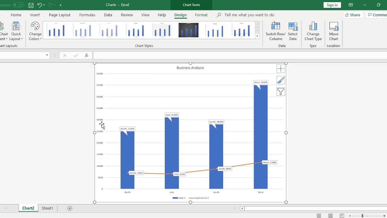
Adding rich data labels to charts in Excel 2013 | Microsoft 365 Blog The data labels up to this point have used numbers and text for emphasis. Putting a data label into a shape can add another type of visual emphasis. To add a data label in a shape, select the data point of interest, then right-click it to pull up the context menu. Click Add Data Label, then click Add Data Callout. The result is that your data label will appear in a graphical callout. How to Add Data Labels to your Excel Chart in Excel 2013 Data labels show the values next to the corresponding chart element, for instance a percentage next to a piece from a pie chart, or a total value next to a column in a column chart. You can choose...

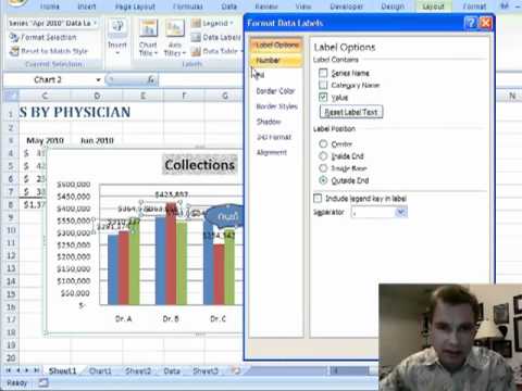
Data Labels in Excel Pivot Chart (Detailed Analysis) Next open Format Data Labels by pressing the More options in the Data Labels. Then on the side panel, click on the Value From Cells. Next, in the dialog box, Select D5:D11, and click OK. Right after clicking OK, you will notice that there are percentage signs showing on top of the columns. 4. Changing Appearance of Pivot Chart Labels

Excel 2013 data labels

Excel Tips n Tricks -Tip 8 (Applying Chart Data Labels From a Range in ... Click on the plus symbol, the first icon, and check "Data Labels". Now you will see them added to your chart. You can also click on the right arrow on "Data Labels" and select where you want the data labels to be aligned, in other words center, right, top, bottom and so on. Picture 4 4. I modified the chart and axis titles to look good. How to Use Cell Values for Excel Chart Labels - How-To Geek Select the chart, choose the "Chart Elements" option, click the "Data Labels" arrow, and then "More Options.". Uncheck the "Value" box and check the "Value From Cells" box. Select cells C2:C6 to use for the data label range and then click the "OK" button. The values from these cells are now used for the chart data labels. Add or remove data labels in a chart - support.microsoft.com To label one data point, after clicking the series, click that data point. In the upper right corner, next to the chart, click Add Chart Element > Data Labels. To change the location, click the arrow, and choose an option. If you want to show your data label inside a text bubble shape, click Data Callout.

Excel 2013 data labels. How to mail merge and print labels from Excel - Ablebits.com Select document type. The Mail Merge pane will open in the right part of the screen. In the first step of the wizard, you select Labels and click Next: Starting document near the bottom. (Or you can go to the Mailings tab > Start Mail Merge group and click Start Mail Merge > Labels .) Choose the starting document. Values From Cell: Missing Data Labels Option in Excel 2013? When a chart created in 2013 using the "Values from Cell" data label option is opened with any earlier version of Excel, the data labels will show as "[CELLRANGE]". If you want to ensure that data labels survive different generations of Excel, you need to revert to the old technique: Insert data labels Edit each individual data label How to hide zero data labels in chart in Excel? - ExtendOffice 1. Right click at one of the data labels, and select Format Data Labels from the context menu. See screenshot: 2. In the Format Data Labels dialog, Click Number in left pane, then select Custom from the Category list box, and type #"" into the Format Code text box, and click Add button to add it to Type list box. See screenshot: 3. Data Labels above bar chart - Excel Help Forum Excel 2013 Posts 191 Data Labels above bar chart Is there a way to have data labels above bar chart even if the data changes. I manually move the labels above but once the data changes I have to adjust. I don't see a setting for this. Register To Reply 06-03-2016, 03:28 AM #2 Andy Pope Forum Guru Join Date 05-10-2004 Location Essex, UK MS-Off Ver

How to Add Total Data Labels to the Excel Stacked Bar Chart Step 4: Right click your new line chart and select "Add Data Labels" Step 5: Right click your new data labels and format them so that their label position is "Above"; also make the labels bold and increase the font size. Step 6: Right click the line, select "Format Data Series"; in the Line Color menu, select "No line" Step 7: Delete the "Total" data series label within the legend Custom Chart Data Labels In Excel With Formulas - How To Excel At Excel Follow the steps below to create the custom data labels. Select the chart label you want to change. In the formula-bar hit = (equals), select the cell reference containing your chart label's data. In this case, the first label is in cell E2. Finally, repeat for all your chart laebls. How to add data labels from different column in an Excel chart? Right click the data series in the chart, and select Add Data Labels > Add Data Labels from the context menu to add data labels. 2. Click any data label to select all data labels, and then click the specified data label to select it only in the chart. 3. How to Add Data Labels in Excel - Excelchat | Excelchat In Labels group, click on Data Labels and select the position to add labels to the chart. Figure 3. Chart Data Labels. Figure 4. How to Add Data Labels. In Excel 2013 And Later Versions. In Excel 2013 and the later versions we need to do the followings; Click anywhere in the chart area to display the Chart Elements button ; Figure 5. Chart Elements Button. Click the Chart Elements button > Select the Data Labels, then click the Arrow to choose the data labels position. Figure 6.

Create Dynamic Chart Data Labels with Slicers - Excel Campus Step 3: Use the TEXT Function to Format the Labels. Typically a chart will display data labels based on the underlying source data for the chart. In Excel 2013 a new feature called "Value from Cells" was introduced. This feature allows us to specify the a range that we want to use for the labels. Custom data labels in a chart - Get Digital Help If you have excel 2013 you can use custom data labels on a scatter chart. 1. Right press with mouse on a series 2. Press with left mouse button on "Add Data Labels" 3. Right press with mouse again on a series 4. Press with left mouse button on "Format Data Labels" 5. Enable check box "Value from cells" 6. Select a cell range 7. Disable check ... Excel 2013 Chart Labels don't appear properly - Microsoft Community You've stumbled on a big problem - Excel 2013 lets you edit data labels directly, but this feature (rich text data labels) is not backwards-compatible and there's no way to turn it off. It's great to be able to modify the text of labels, or direct them to get contents from a worksheet cell. Custom Data Labels with Colors and Symbols in Excel Charts - [How To ... To apply custom format on data labels inside charts via custom number formatting, the data labels must be based on values. You have several options like series name, value from cells, category name. But it has to be values otherwise colors won't appear. Symbols issue is quite beyond me.

How to Add Data Labels in Excel - Excelchat | Excelchat

How to insert data labels to a Pie chart in Excel 2013 - YouTube This video will show you the simple steps to insert Data Labels in a pie chart in Microsoft® Excel 2013. Content in this video is provided on an "as is" basi...

How to Add Data Labels to your Excel Chart in Excel 2013 - YouTube

Quick Tip: Excel 2013 offers flexible data labels | TechRepublic With the cursor inside that data label, right-click and choose Insert Data Label Field. In the next dialog, select. [Cell] Choose Cell. When Excel displays the source dialog, click the cell that ...

How To Add Data Labels To A Chart in Microsoft Excel - YouTube

Change the format of data labels in a chart To get there, after adding your data labels, select the data label to format, and then click Chart Elements > Data Labels > More Options. To go to the appropriate area, click one of the four icons ( Fill & Line, Effects, Size & Properties ( Layout & Properties in Outlook or Word), or Label Options) shown here.

Surface Chart in Excel

Excel Data Labels - Value from Cells I created a chart and linked the data labels to a series of cells, as 2013 allows in Value From Cells option. I pre-select e.g. 100 data rows even though it initially contains values in 10 of them. When I reopen the workbook and add x and y value and a new label (where I left empty cells to do so) that data point 'icon' comes on to the graph ...

Excel Video 77 Data Labels - YouTube

Excel Data Labels - Microsoft Community I created a chart and linked the data labels to a series of cells, as 2013 allows in Value From Cells option. fyi: The data labels are names of individuals, and the data points (x,y numbers) are in two other columns. I create this to use as a template (but not Saved As a "template" proper).

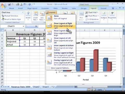
How to add or remove legends, titles or data labels in MS Excel - YouTube

Change the format of data labels in a chart To format data labels, select your chart, and then in the Chart Design tab, click Add Chart Element > Data Labels > More Data Label Options. Click Label Options and under Label Contains , pick the options you want.

Creating Mailing Labels Using The Mail Merge Helper In MS Word 2003 - Library & ITS Wiki

How to Print Labels from Excel - Lifewire To label legends in Excel, select a blank area of the chart. In the upper-right, select the Plus ( +) > check the Legend checkbox. Then, select the cell containing the legend and enter a new name. How do I label a series in Excel? To label a series in Excel, right-click the chart with data series > Select Data.

Waterfall Chart - Page 2 of 2 - Beat Excel!

Add Custom Labels to x-y Scatter plot in Excel Step 1: Select the Data, INSERT -> Recommended Charts -> Scatter chart (3 rd chart will be scatter chart) Let the plotted scatter chart be. Step 2: Click the + symbol and add data labels by clicking it as shown below. Step 3: Now we need to add the flavor names to the label. Now right click on the label and click format data labels.

Microsoft Excel 2013 Tutorial - Learn New Features in Excel 2013 | IT Online Training

Custom Chart Labels Using Excel 2013 | MyExcelOnline View the Benchmark Chart using Excel 2013. DOWNLOAD EXCEL WORKBOOK. STEP 1: We added a % Variance column in our data and inserted symbols to show a negative and positive variance. ** You can see the tutorial of how this is done here **. STEP 2: In our graph we need to select the Sales chart and Right Click and choose Add Data Labels.

Show Trend Arrows in Excel Chart Data Labels

Format Data Labels in Excel- Instructions - TeachUcomp, Inc. To format data labels in Excel, choose the set of data labels to format. To do this, click the "Format" tab within the "Chart Tools" contextual tab in the Ribbon. Then select the data labels to format from the "Chart Elements" drop-down in the "Current Selection" button group.

How to Print Labels from Excel

Add or remove data labels in a chart - support.microsoft.com To label one data point, after clicking the series, click that data point. In the upper right corner, next to the chart, click Add Chart Element > Data Labels. To change the location, click the arrow, and choose an option. If you want to show your data label inside a text bubble shape, click Data Callout.

How to Mail Merge using Microsoft Excel and Word - YouTube

How to Use Cell Values for Excel Chart Labels - How-To Geek Select the chart, choose the "Chart Elements" option, click the "Data Labels" arrow, and then "More Options.". Uncheck the "Value" box and check the "Value From Cells" box. Select cells C2:C6 to use for the data label range and then click the "OK" button. The values from these cells are now used for the chart data labels.