41 update data labels in excel chart
Modify chart legend entries - support.microsoft.com On the worksheet, click the cell that contains the name of the data series that appears as an entry in the chart legend. Type the new name, and then press ENTER. The new name automatically appears in the legend on the chart. Edit legend entries in the Select Data Source dialog box Excel.Interfaces.ChartDataLabelsUpdateData interface - Office Add-ins ... excel An interface for updating data on the ChartDataLabels object, for use in chartDataLabels.set ( { ... }). In this article Properties Property Details Properties Property Details auto Text Specifies if data labels automatically generate appropriate text based on context. TypeScript Copy autoText?: boolean; Property Value boolean Remarks
Excel.Interfaces.ChartDataLabelUpdateData interface - Office Add-ins ... Represents the horizontal alignment for chart data label. See Excel.ChartTextHorizontalAlignment for details. This property is valid only when TextOrientation of data label is -90, 90, or 180. left: Represents the distance, in points, from the left edge of chart data label to the left edge of chart area. Value is null if the chart data label is ...

Update data labels in excel chart
Data Labels in Excel Pivot Chart (Detailed Analysis) Click on the Plus sign right next to the Chart, then from the Data labels, click on the More Options. After that, in the Format Data Labels, click on the Value From Cells. And click on the Select Range. In the next step, select the range of cells B5:B11. Click OK after this. Label Values not updating, but chart is? - MrExcel Message Board I am having the same problem -- now in Excel 2007 -- and turning the labels on and off did the trick! Since this thread is old, here is an update for folks using XL '07: start by right-clicking the chart, selecting "Format Data Labels" from the menu. Under the "Label Options" tab there is a button for "Reset Label Text". Change the format of data labels in a chart To get there, after adding your data labels, select the data label to format, and then click Chart Elements > Data Labels > More Options. To go to the appropriate area, click one of the four icons ( Fill & Line, Effects, Size & Properties ( Layout & Properties in Outlook or Word), or Label Options) shown here.
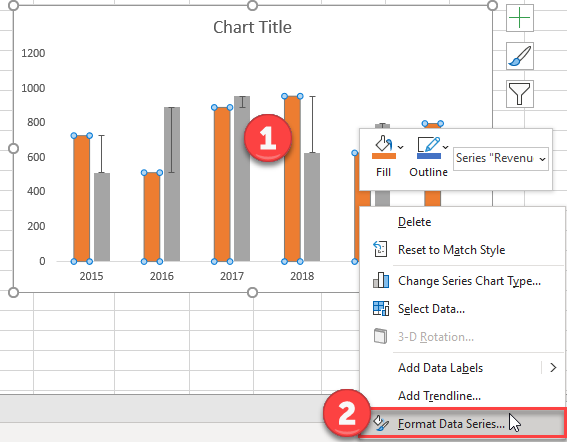
Update data labels in excel chart. Changing data label format for all series in a pivot chart To change data labels format, please perform the following steps: Click the pivot chart > + sign near tthe pivot chart > right click data label of any series > Format Data Series... Edit titles or data labels in a chart - support.microsoft.com The first click selects the data labels for the whole data series, and the second click selects the individual data label. Right-click the data label, and then click Format Data Label or Format Data Labels. Click Label Options if it's not selected, and then select the Reset Label Text check box. Top of Page Display Data Labels Above Data Markers in Excel Chart We use the following steps: Activate the chart by clicking just below the top boundary of the chart. The Chart Elements button, with a green cross icon, appears at the top right corner of the chart.. Click the Chart Elements button and check the Data Labels check box. Data labels immediately appear on top of the data markers in the chart. Chart.ApplyDataLabels method (Excel) | Microsoft Learn The type of data label to apply. True to show the legend key next to the point. The default value is False. True if the object automatically generates appropriate text based on content. For the Chart and Series objects, True if the series has leader lines. Pass a Boolean value to enable or disable the series name for the data label.
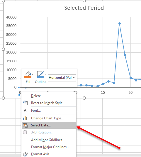
Add / Move Data Labels in Charts - Excel & Google Sheets Check Data Labels . Change Position of Data Labels. Click on the arrow next to Data Labels to change the position of where the labels are in relation to the bar chart. Final Graph with Data Labels. After moving the data labels to the Center in this example, the graph is able to give more information about each of the X Axis Series. Excel Chart - Selecting and updating ALL data labels - Right-click a "point" in the series, which actually will be a bar piece - Choose add data labels - Right-click again and choose format data labels - Check series name - Uncheck value That's it…. You must log in or register to reply here. Similar threads S Data Labels disappearing off excel chart Sundance_Kid Aug 21, 2022 Excel Questions Replies 0 Labels of embedded chart in powerpoint won't update 1. create a diagram in excel an copy it to a PowerPoint sheet, update links between the documents are enabled automatically. 2. if new data needs to be added: right click the chart, add data (I'm not sure if thats the right translation) - an excel window pops up. The new data point is shown in the chart, the new label is only shown as empty box. Update the data in an existing chart - support.microsoft.com Try it! Changes you make will instantly show up in the chart. Right-click the item you want to change and input the data--or type a new heading--and press Enter to display it in the chart.. To hide a category in the chart, right-click the chart and choose Select Data.. Deselect the item in the list and select OK.. To display a hidden item on the chart, right-click and Select Data and reselect ...
Add or remove data labels in a chart - support.microsoft.com Click the data series or chart. To label one data point, after clicking the series, click that data point. In the upper right corner, next to the chart, click Add Chart Element > Data Labels. To change the location, click the arrow, and choose an option. If you want to show your data label inside a text bubble shape, click Data Callout. Data labels move when graph data updates - Microsoft Community I'm having issues with a graph I've made in excel. It's a doughnut graph which has the data labels right where the angle of the first slice is (at the top of the graph plot area). The issue is that when the data flowing into the graph is updated, the labels jump to somewhere new on the graph. How can I stop this from happening? Thanks! Change the format of data labels in a chart To get there, after adding your data labels, select the data label to format, and then click Chart Elements > Data Labels > More Options. To go to the appropriate area, click one of the four icons ( Fill & Line, Effects, Size & Properties ( Layout & Properties in Outlook or Word), or Label Options) shown here. Label Values not updating, but chart is? - MrExcel Message Board I am having the same problem -- now in Excel 2007 -- and turning the labels on and off did the trick! Since this thread is old, here is an update for folks using XL '07: start by right-clicking the chart, selecting "Format Data Labels" from the menu. Under the "Label Options" tab there is a button for "Reset Label Text".
How to Add Data Labels to your Excel Chart in Excel 2013
Data Labels in Excel Pivot Chart (Detailed Analysis) Click on the Plus sign right next to the Chart, then from the Data labels, click on the More Options. After that, in the Format Data Labels, click on the Value From Cells. And click on the Select Range. In the next step, select the range of cells B5:B11. Click OK after this.
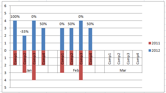
Add % Difference Data Labels to Excel Horizontal Tornado ...
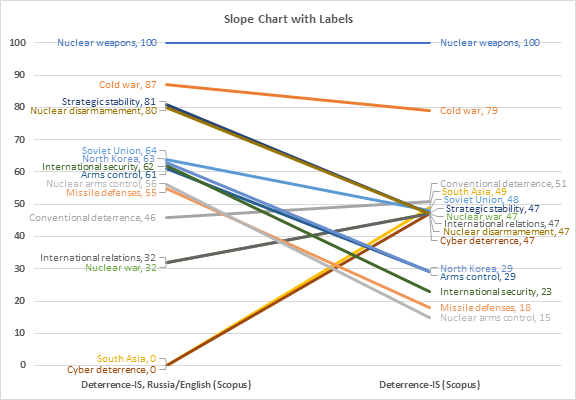
Slope Chart with Data Labels - Peltier Tech

How to change data labels in a bar chart? : r/excel
How-to Add Custom Labels that Dynamically Change in Excel ...

Adding Data Labels to Your Chart (Microsoft Excel)

Add or remove data labels in a chart

Add data labels and callouts to charts in Excel 365 ...

Adding rich data labels to charts in Excel 2013 | Microsoft ...

Change the format of data labels in a chart

Adding rich data labels to charts in Excel 2013 | Microsoft ...

Change the format of data labels in a chart

excel - VBA Change Data Labels on a Stacked Column chart from ...

Google Workspace Updates: Get more control over chart data ...

Dynamically Label Excel Chart Series Lines • My Online ...

How to Get Colors in Excel Chart Data Lables - Formatting Trick

How to add live total labels to graphs and charts in Excel ...

Custom Excel Chart Label Positions • My Online Training Hub

Add Labels ON Your Bars

Format Number Options for Chart Data Labels in PowerPoint ...

How to add or move data labels in Excel chart?

How to Customize Your Excel Pivot Chart Data Labels - dummies

Custom data labels in a chart
Change Horizontal Axis Values in Excel 2016 - AbsentData

How to Add Data Labels to an Excel 2010 Chart - dummies

How to add data labels from different column in an Excel chart?

How to Add Two Data Labels in Excel Chart (with Easy Steps ...

Google Workspace Updates: Directly click on chart elements to ...

Excel charts: add title, customize chart axis, legend and ...
Is there a way to change the order of Data Labels ...

How to Add Data Labels in Excel - Excelchat | Excelchat

How to add live total labels to graphs and charts in Excel ...

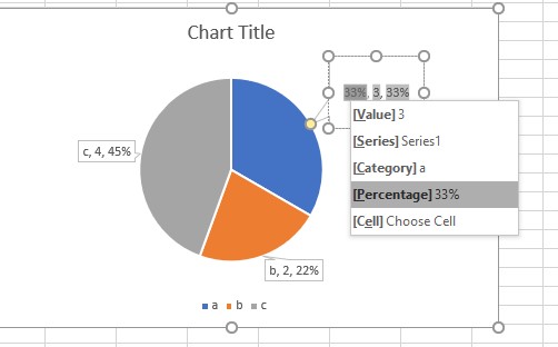
Is there a way to add data labels as percentages on the ...
Move and Align Chart Titles, Labels, Legends with the Arrow ...
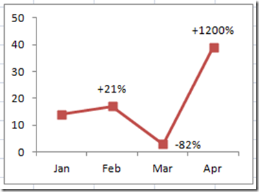
Percentage Change Chart – Excel – Automate Excel

Creating Pie Chart and Adding/Formatting Data Labels (Excel)

Change the format of data labels in a chart

How to add or move data labels in Excel chart?
Change Horizontal Axis Values in Excel 2016 - AbsentData

Highlight a Specific Data Label in an Excel Chart - Peltier Tech

Add data labels and callouts to charts in Excel 365 ...
Post a Comment for "41 update data labels in excel chart"